Isotopes and convention for reporting isotope data
Elements in nature come in forms called isotopes that differ only in the number of their neutrons. Most isotopes are stable and can be distinguished from their counterparts simply by their masses. Stable isotopes are denoted by their atomic mass such as ¹³C and ¹²C for the two stable isotopes of carbon, and ¹⁸O, ¹⁷O, and ¹⁶O for the stable isotopes of oxygen. Isotopes are species of a chemical element which differ from one another by atomic weight. The abundances of carbon and oxygen isotopes in nature are:

These isotopes are of pivotal interest because they vary in natural substances as a function of processes such as photosynthesis, evaporation, precipitation, cementation and can therefore be used as tracers of these processes. Because the heavy isotope is normally rare, routine measurements of the absolute isotopic concentrations is difficult and not reliable. Alternatively, the ratio, R, of the rare to the abundant isotopes is measured, such as ¹³R = ¹³C/¹²C for carbon or ¹³R = ¹⁸O/¹⁶O for oxygen.
To reduce variations due to instrumental drifts and instabilities, the common procedure in stable isotope analyses is to compare the ratio in a sample to that of a standard that is assumed to have a constant and known isotopic ratio. Isotope ratios are therefore reported in their normalized difference form as “delta values” where

As shown by these equations, the δ value is a relative difference between a sample (R_Sample) and a standard (R_Standard), and is a dimensionless parameter. Since values of δ in nature are small, they are generally given in ‰ (per mil) – which is a 10³ factor, not a unit. Further, only the arbitrary choice of standard determines whether a δ value of a sample is positive or negative (Mook, 2000). The ¹⁸O/¹⁶O ratio (or ¹³C/¹²C ratio) is smaller in the sample than in the standard, then the sample is depleted in the ¹⁸O (or ¹³C, respectively) relative to the standard and the δ value is a negative number. Conversely, if the ¹⁸O/¹⁶O ratio (or ¹³C/¹²C ratio) is larger in the sample than in the standard, then the sample is enriched in ¹⁸O (or ¹³C, respectively) relative to the standard, and its δ value is a positive number. To allow efficient comparisons of results among different labs around the world, a series of common international standards has been established and all samples are normalized to such standards. For carbon, the common standard was originally a carbonate of the Pee Dee belemnite carbonate formation in South Carolina. Naturally, as the original standards are exhausted, appropriate substitutes have been introduced. The two main sources for international standards today are the International Atomic Energy Association (IAEA - https://www.iaea.org/) in Vienna, and the US National Institute of Standards and Technology (NIST - https://www.nist.gov/).

Mid-Infrared Spectroscopy for CO₂ Isotopologue Analysis
Within the field of physics, electromagnetic radiation embodies waves within the electromagnetic field, traversing space while carrying both momentum and electromagnetic radiant energy. The electromagnetic spectrum comprehensively encloses various forms of electromagnetic radiation, such as radio waves, microwaves, infrared, visible light, ultraviolet, X-rays, and gamma rays. Each segment of this spectrum engages in distinct interactions with matter, offering diverse applications in various scientific and technological fields.

Consider a white beam source, emitting light across multiple wavelengths, focused onto a sample, such as amorphic glass. When this beam interacts with the sample, photons matching the energy gap of the molecules present are selectively absorbed to excite these molecules. Simultaneously, other photons remain unaffected and transmit through. In cases where the radiation falls within the visible region (400–700 nm), the color of the sample becomes the complementary color of the absorbed light. Absorption spectroscopy serves as a vital analytical chemistry tool, adept at discerning the presence of specific substances in a given sample. Furthermore, it often enables the quantification of the amount of the substance under scrutiny. Both infrared and ultraviolet–visible spectroscopy are notably prevalent in analytical applications, exemplifying the versatility of absorption spectroscopy across diverse scientific disciplines.
The absorption intensity, varying with the frequency of electromagnetic radiation, gives rise to the absorption spectrum. This phenomenon is harnessed through absorption spectroscopy across the electromagnetic spectrum.

The utility of absorption spectroscopy in chemical analysis lies in its specificity and quantitative attributes. The specificity enables the differentiation of compounds within mixtures, making absorption spectroscopy applicable across a wide range of fields. Moreover, the specificity facilitates the identification of unknown samples by comparing measured spectra with a reference library. Even in cases where a library match is absent, qualitative information about a sample can be deduced. For example, infrared spectra exhibit characteristic absorption bands indicating the presence of specific bonds, such as carbon-hydrogen or carbon-oxygen. Recent technological strides in spectroscopy have enabled the discrimination of various isotopologues of CO₂, treating them as distinct entities. CO₂ isotopologues, resulting from the replacement of common isotopes ¹²C and ¹⁶O of carbon and oxygen with the less common ¹³C and ¹⁸O, exhibit unique absorption spectra in the mid-infrared range. The substitution of an atom by a heavier isotope, such as ¹³C replacing ¹²C or ¹⁸O replacing ¹⁶O, induces a spectrum shift, allowing for the differentiation between the two isotopologues. Key isotopologues of CO₂ include ¹²C¹⁶O¹⁶O (mass 44), ¹³C¹⁶O¹⁶O (mass 45), and ¹²C¹⁶O¹⁸O (mass 46). Quantized rotational and vibrational states generate a distinctive spectral fingerprint. Determining the ratio of peaks from selected regions of the spectrum enables the accurate simultaneous measurement of ¹³C and ¹⁸O of CO₂. Absorptions for CO₂ are notably stronger in the mid-infrared compared to the near-infrared, allowing for the application of simple direct absorption approaches to achieve high specificity, sensitivity, and accuracy.

Measurement Method
The differentiation of the three main CO₂ isotopologues (with masses 44, 45, and 46) in the air is based on measurements of mid-infrared light absorption (λ ≈ 4.3 μm) and subsequent concentration calculation using the Lambert–Beer law. The analyzer collects measurements at 1 Hz, determining the ¹³C/¹²C ratio, ¹⁸O/¹⁶O ratios, and CO₂ concentration. Laser-based analyzers offer advantages over more complex methods, such as IRMS, as CO₂ sample purification is unnecessary, enabling high-frequency measurements of isotopic ratios. This method proves valuable in studying atmospheric CO₂ patterns. Isotope analyzers automatically manage working standard gases for calibration, referencing measurements against isotopic working standards. Referencing is conducted hourly to achieve high precision and accuracy (σ = ± 0.25‰ for both δ¹³C and δ¹⁸O). A calibration procedure correlates the analytical signal with the ¹³C/¹²C and ¹⁸O/¹⁶O ratios of working standards. Pure CO₂ (purity >99.999 vol. %) with known ¹³C/¹²C and ¹⁸O/¹⁶O ratios against international standards serves as the reference. 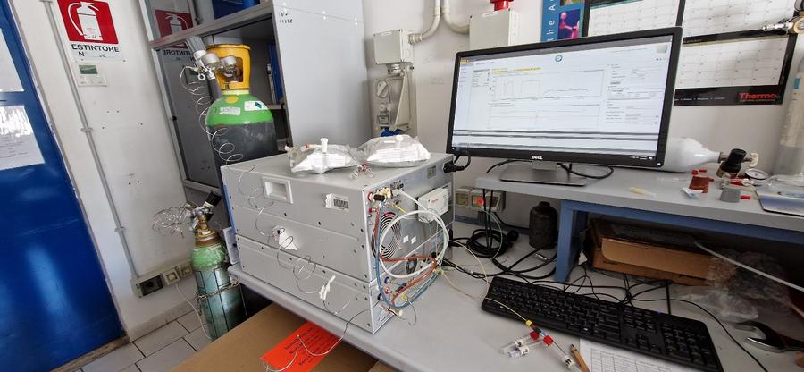For atmospheric gas collection, a stainless-steel capillary is utilized, fixed outside the Istituto Nazionale di Geofisica e Vulcanologia in Palermo (13.60 m above the ground floor).

Environmental variables, including air temperature, atmospheric pressure, relative humidity, rain rate, radiation, evapotranspiration, wind direction, and wind speed, are also measured. These variables play a crucial role in investigating pollutant patterns, especially regarding gas dispersion. Collected by a weather station on the roof of the ACO-Laboratory, the data avoids interference with surrounding buildings and provides insights into air circulation at the site of air CO₂ monitoring. The station records all parameters with a 5-minute sampling frequency.

Hints on Gas Emission Origins through Stable Isotopic Composition
A thorough examination of the origins of gas emissions is attainable through the application of stable isotopic composition analysis, employing the Keeling plot approach. This methodology aids in understanding the sources contributing to atmospheric CO₂ emissions by comparing isotopic data against the inverse of CO₂ concentration. Rooted in a two-component mixing model, the Keeling plot presents a linear combination of isotopic mass balance, resulting in straight lines within the δ¹³C vs. 1/C plot (Keeling, 1958; Pataki et al., 2003). Both δ¹³C and δ¹⁸O play pivotal roles in distinguishing processes involving atmospheric CO₂. While δ¹³C reveals information about CO₂ sources, δ¹⁸O tracks CO₂ fluxes through geospheres.

The keeling plot (see the above figure) shows the mixing lines between atmospheric CO₂ and several sources of CO₂ in the atmosphere either natural or anthropogenic. Line “Natural gas CO₂” represents the addition of CO₂ from combustion of natural gas (δ¹³C = -42‰ VPDB); Line “Fossil fuel combustion CO₂” represents the addition of CO₂ from combustion of petroleum (δ¹³C = -27‰ VPDB); Line “Soil/Plant respired CO₂” represents the addition of CO₂ from soil respiration (δ¹³C = -25.7‰ VPDB); Line “Volcanic Plume” represents the addition of CO₂ from volcanic degassing (δ¹³C = +4.0‰ VPDB); Line “Ocean/Atmosphere” represents the addition of CO₂ from ocean-atmosphere equilibrium (δ¹³C = +0.2‰ VPDB); Line “Landfill CO₂ emissions” represents the addition of CO₂ from waste decomposition (δ¹³C = +20.0‰ VPDB). Blue line shows the evolution of stable isotopes in CO₂ and CO₂ concentration between a Holocene pre-industrial atmospheric CO₂ and the approximate global atmospheric CO₂ at early XX1 century (380 ppm vol). For reference, the dashed line was extrapolated to CO₂ concentrations higher than those of modern global atmospheric CO₂.
The intercepts on the straight line in above figure indicates the carbon isotope composition of a variety of sources of CO₂. The Keeling method offers insight into the isotopic signature of the CO₂ source, under the assumption of constancy in both background and CO₂ sources throughout the observation period. Urban zones, characterized by diverse human activities, present complex systems where various emissions contribute to the isotope composition in the atmosphere. In specific localities, geological outgassing, such as active or extinct volcanic degassing, emerges as the primary source of CO₂ emissions.

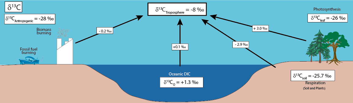
Annual mean forcings on the δ¹³C value of atmospheric CO₂ (see the above figure after Yakir, 2003). Each specific forcing component represents the product of the involved flux, diluted by the atmospheric carbon pool, and the difference in δ¹³C values between the flux and the mean atmosphere. The values presented are order-of-magnitude estimates, as elaborated in the text, and entail notable uncertainties. The typical values for the relevant carbon reservoirs are provided in the accompanying boxes. Among these, the land biosphere exerts the most substantial forcing, driven by the contrasting impacts of photosynthesis and respiration. The net photosynthetic carbon sink tends to enrich the atmosphere in ¹³C. Comparatively, the oceanic forcing is nearly an order of magnitude smaller than the land effect, establishing a foundation for distinguishing between land and ocean sinks and sources. Fossil fuel emissions, conversely, act to dilute atmospheric ¹³C. Despite the nearly balanced nature of these distinct forcings, the fossil fuel effect emerges as the dominant contributor to atmospheric forcing, resulting in a net trend of 0.02‰ per year. The interplay of these forcing components showcases the complex dynamics within the carbon cycle, underscoring the importance of acknowledging the uncertainties inherent in such estimations. The δ¹⁸O signal demonstrates a unique coupling between the hydrological and carbon cycles, reflecting the exchange of CO₂ with the terrestrial biosphere. The global δ¹⁸O background signal, established by atmosphere-ocean water exchange, undergoes modification on land through interactions with the biosphere (Ciais and Maijer, 1998). Oxygen atom replacement processes in atmospheric CO₂ involve exchanges with water in seawater, soils, and plant leaves. CO₂-H₂O oxygen exchange in plant leaves, where carbonic anhydrase facilitates the equilibration of ¹⁸O content, transfers this signal to air CO₂. The hydration of CO₂ molecules, a crucial process for oxygen exchange, occurs slowly at 25 °C, primarily involving reactions with water and carbonic anhydrase in plant leaves (Mills and Urey, 1940). The isotopic equilibration does not occur in the atmosphere due to limited liquid water content, acting as a rate-limiting variable. Soil respiration, catalyzed by carbonic anhydrase in soils, introduces an alternative process affecting δ¹⁸O, with contrasting effects from photosynthesis.

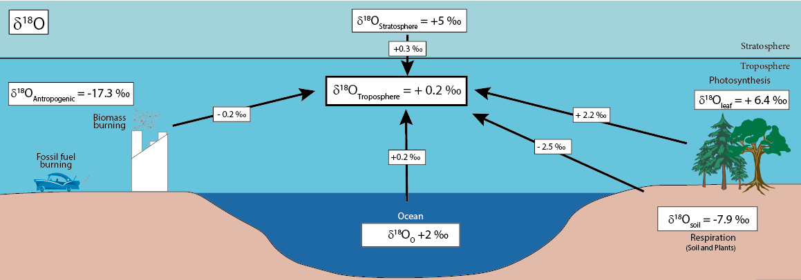
Annual mean "forcings" on the δ¹⁸O value of atmospheric CO₂ delineate the impact of various influencing factors (see the above figure after Yakir, 2003). Each specific forcing component results from the product of the involved flux, diluted by the atmospheric carbon pool, and the difference in δ¹⁸O values between the flux and the mean atmosphere. The values presented are order-of-magnitude estimates, as detailed in the text, and are subject to significant uncertainties. The typical values for the involved reservoirs are provided in accompanying boxes, reflecting the δ¹⁸O value of the water in each reservoir. Notably, the anthropogenic reservoir is represented by the δ¹⁸O value of atmospheric oxygen.
Among these forcings, the land biosphere emerges as the most influential, marked by the contrasting effects of photosynthesis and respiration. Land photosynthesis tends to enrich the atmosphere in ¹⁸O, while soil respiration has the opposite effect. This dichotomy provides a foundation for distinguishing between the fluxes of photosynthesis and respiration. In contrast, the oceanic forcing is an order of magnitude smaller. Fossil fuel emissions, meanwhile, act to decrease ¹⁸O, yet this effect is often "washed away" by the substantial exchange of oxygen in CO₂ with water. As a result, a discernible long-term trend in the atmospheric δ¹⁸O is not commonly observed. The intricate interplay of these forcings underscores the complexity of factors influencing the isotopic composition of atmospheric CO₂, necessitating an acknowledgment of the inherent uncertainties in these estimations. Interpreting δ¹⁸O can be complex, but frequent measurements with high precision offer insights into local CO2 source values. While uncertainties may arise, the Keeling plot method aids in retrieving δ¹⁸O, considering factors such as soil respiration and plant photosynthesis, providing valuable information about the local source's isotopic composition.